1. Why a New File Format?
Apache Parquet has been the undisputed king of analytical columnar storage for over a decade. So why did the LanceDB team invest years building Lance from scratch?
The answer lies in a fundamental mismatch: Parquet was designed for OLAP scan workloads on tabular data; the AI era demands something different.
The Three Forces Driving a New Format
A) Random Access at Scale
Parquet achieves great compression and scan throughput through row groups blocks of rows that are compressed together. But this design makes point lookups expensive. To read a single row, you must decompress an entire page (often 1 MB+). When your workflow is vector search (finding the top k nearest neighbours out of millions of vectors), you're essentially doing millions of such point lookups. Parquet is structurally ill suited to this access pattern.
Lance is benchmarked at ~100× faster random access than Parquet. It achieves this by ensuring every encoding is "sliceable" you can extract a single value without decoding its entire page.
B) Multimodal & Wide Data
Traditional databases store strings and floats. ML workloads store:
- High dimensional embeddings (e.g., 1536 float CLIP vectors ≈ 6 KiB per row)
- Raw image bytes (100 KB–10 MB per row)
- 3D point clouds, audio waveforms, video frames
Parquet's row group sizing becomes a nightmare here. A row group sized for small floats will be comically large when each row contains a 4 MB image, and one sized for images will be tiny for float columns. There is no good universal choice.
C) Unified Storage for Original Data + Embeddings
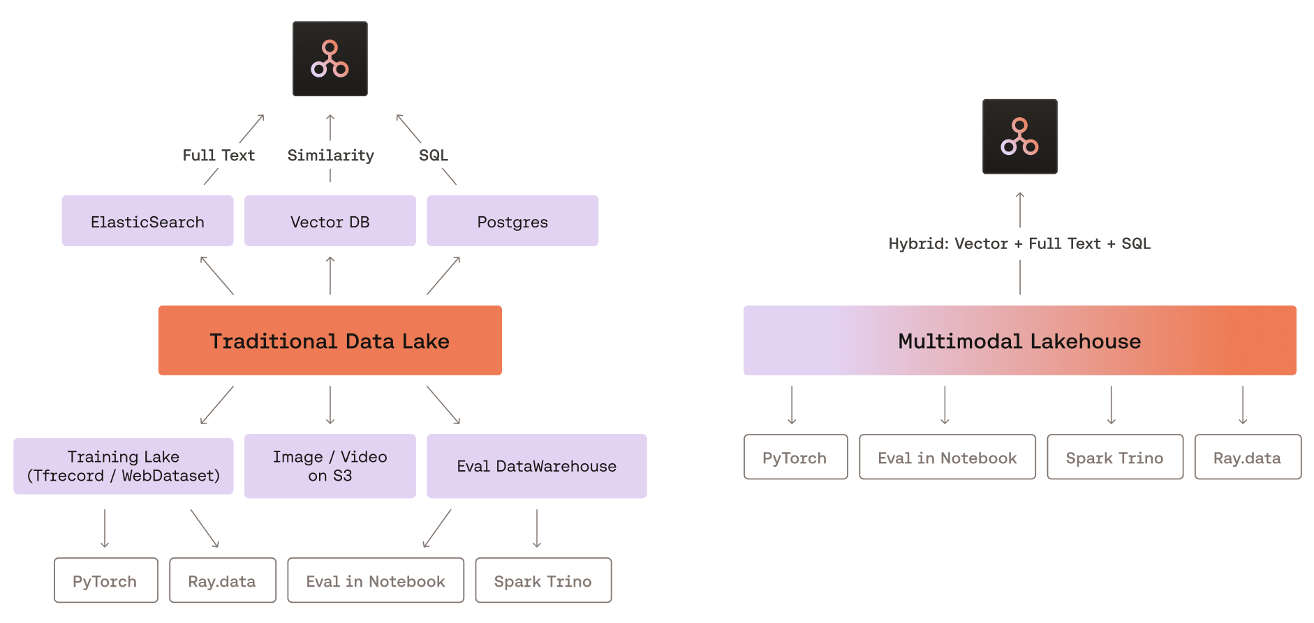
Most vector database architectures force a split: store your raw data (images, docs) somewhere like S3, then store only the embeddings + metadata in the vector DB. This adds operational complexity, latency, and cost. Lance stores original data and its vector representations together in the same format, acting as a unified multimodal lakehouse.
What Parquet Does Wrong (Technically)
Parquet File
├── Row Group 0  (e.g., rows 0–65535)
│   ├── Column Chunk: "id"
│   │   ├── Page 0  [compressed, must decompress all to get row 42]
│   │   └── Page 1
│   ├── Column Chunk: "embedding"
│   │   └── Page 0  [128 KiB compressed; a single value is buried inside]
│   └── ...
├── Row Group 1
└── File Footer   [ALL column metadata expensive for wide schemas]
Key Parquet pain points:
- Row groups create a "one size fits none" problem for mixed workloads
- Encodings can't access column/file metadata, forcing redundant data (e.g., dictionaries repeated per row group instead of stored once)
- Page level access granularity means reading one value reads an entire page
- Wide schema metadata must be fully read even when projecting a single column
- Adding new encodings requires modifying every reader implementation across the ecosystem
2. Lance vs. Parquet: Side-by-Side
| Feature | Apache Parquet | Lance (v2.1) |
|---|---|---|
| Primary Design Goal | OLAP analytics, ETL | ML/AI workloads, ANN search, multimodal |
| Access Pattern | Sequential scan | Both sequential scan and random access |
| Row Groups | Yes (fundamental unit, 64K–128K rows typical) | No (eliminated entirely in v2) |
| Random Access Speed | Slow (must decode entire page) | ~100× faster; direct offset calculation |
| Compression | Aggressive (Snappy, Zstd, Gzip) | Structural + compressive encodings (v2.1); avoids sacrificing random access |
| Embedding/Tensor Storage | Awkward (requires fixed size list tricks) | First class; wide columns handled natively |
| Versioning | None (external tooling, e.g., Delta Lake) | Built in, zero copy versioning (Git-like) |
| Vector Index | None | IVF-PQ, IVF-HNSW-PQ, IVF-HNSW-SQ, binary |
| Full Text Search | None | Yes (inverted index built in) |
| Deletions | Rewrite entire file | Soft delete via deletion file per fragment |
| Schema Evolution | Partial support | Full; tracked per version |
| Encoding Extensibility | Hard (requires patching readers) | Pluggable; encodings are self describing |
| Ecosystem | Pandas, Spark, Hive, Trino, Athena, ... | Arrow, DuckDB, Pandas, PyTorch, HuggingFace |
| Metadata on Wide Schemas | Full schema loaded always | Lazy; only requested columns' metadata loaded |
| Null Handling | Some edge cases lost (old v1 Lance too) | Explicit null tracking (v2) |
| Storage Format | Single file per partition | Fragments (data files + optional deletion file) + manifest |
| Best For | Data warehousing, BI dashboards, ETL | Vector search, RAG, ML training, feature stores |
3. Lance File Layout & Random Access Internals
3.1 The Dataset Anatomy
A Lance dataset on disk looks like this:
my_dataset.lance/
├── _latest.manifest          ← symlink/pointer to newest version
├── _versions/
│   ├── 1.manifest            ← Version 1 metadata
│   ├── 2.manifest            ← Version 2 metadata (after insert)
│   └── 3.manifest            ← Version 3 metadata (after delete)
├── data/
│   ├── fragment_0/
│   │   ├── data_0.lance      ← Column data file
│   │   └── deletions.bin     ← Roaring bitmap of deleted row IDs
│   ├── fragment_1/
│   │   └── data_0.lance
│   └── fragment_2/
│       └── data_0.lance
└── _indices/
    └── ivf_pq_index/         ← Pre built ANN index files
Manifest = the "table of contents" of the dataset. It tracks which fragments exist, their row counts, schema, and which deletion files apply.
Fragments = immutable chunks of data. Each insert creates one or more new fragments. Fragments are never mutated in place; deletions are tracked in a separate roaring bitmap file. This is the core of Lance's MVCC (multi version concurrency control) design.
3.2 Inside a Lance Data File (v2)
Lance File (v2)
┌─────────────────────────────────────────────┐
│  Column Buffers (contiguous per column)     │
│                                             │
│  [col0_buf0][col0_buf1]...[col1_buf0]...    │
│                                             │
│  Each buffer: encoded values, self-described│
│  by structural encoding metadata            │
│                                             │
├─────────────────────────────────────────────┤
│  Column Metadata Section                    │
│  ┌─────────────────────────────────────┐    │
│  │ col0: { encoding, buffer_offsets[] }│    │
│  │ col1: { encoding, buffer_offsets[] }│    │
│  │ col2: { encoding, buffer_offsets[] }│    │
│  └─────────────────────────────────────┘    │
│  (One entry per column; offset table        │
│   allows O(1) seek to any column)           │
│                                             │
├─────────────────────────────────────────────┤
│  Page Table  (row → buffer offset mapping)  │
│  row 0   → offset 0x000000                  │
│  row 1   → offset 0x000180   ← direct seek  │
│  row N   → offset 0xABCDEF                  │
├─────────────────────────────────────────────┤
│  File Footer (tiny; points to above)        │
└─────────────────────────────────────────────┘
Key insight: unlike Parquet's page based grouping, Lance's page table stores a per row (or per small batch) offset for each column. To read row 42 of the embedding column:
- Load the footer (tiny, cached after first read).
- Look up row 42's offset in the page table an O(1) in memory lookup.
- Issue a single, precise
pread()or range HTTP GET to the byte offset. - Decode only those bytes no wasted decompression.
For fixed width types like int64 or float32, the offset can even be calculated arithmetically (offset = base + rowid × elementsize) without a lookup at all.
3.3 Structural vs. Compressive Encoding (v2.1)
A key innovation in v2.1 is separating two previously conflated concerns:
- Structural encoding: How an array is split into buffers. For example, a list column is split into an offsets buffer and a values buffer. This must be understood to perform slicing/random access.
- Compressive encoding: How each buffer's bytes are compressed (Zstd, BitPack, Delta, RLE, etc.). This is applied after structural encoding and does not affect sliceability.
Array  →  [Structural Encoding]  →  Buffers  →  [Compressive Encoding]  →  Compressed Buffers
                   ↑                                        ↑
            Knows how to                            Pure compression;
            split & reassemble                      does not need to
            for random access                       understand data shape
This separation is what allows Lance v2.1 to have both compression and fast random access the structural layer handles slicing independently of whatever compression is applied beneath.
4. Index Internals: From Memory to Disk
A defining architectural choice of LanceDB is its disk first indexing philosophy. Most vector databases (Qdrant, Weaviate, Milvus) keep HNSW graphs in RAM. LanceDB keeps indexes on disk and uses Lance's fast random access to make that practical.
4.1 IVF-PQ: The Workhorse Disk Index
IVF-PQ combines two techniques: Inverted File (IVF) for partitioning and Product Quantization (PQ) for compression.
Phase 1 — Training (offline, one time)
All Vectors (N × D)
        │
        ▼
   K-Means Clustering
        │
        ▼
  num_partitions Centroids   ← stored on disk
  (e.g., 256 centroids for 256 Voronoi cells)
        │
        ▼
  PQ Codebook Training
  D dimensions split into M subspaces (num_sub_vectors)
  K-means on each subspace → 256 codewords per subspace
  Each vector: M × 1 byte codes instead of D × 4 bytes
  Compression ratio: (D × 4) / M  e.g., 1536 dim → 96 bytes (16× smaller)
Phase 2 — Index Structure on Disk
_indices/ivf_pq/
├── centroids.bin        ← num_partitions × D float32 (small, fits in RAM)
├── pq_codebook.bin      ← M × 256 × (D/M) float32 subspace codewords
└── partition_{i}.lance  ← For each partition: row_ids + PQ codes
                            of vectors assigned to centroid i
Phase 3 — Query Time
Query Vector q (D dimensional)
        │
   [In Memory]
   1. Compute distance from q to all num_partitions centroids
   2. Select top nprobes closest centroids
        │
   [Disk I/O — targeted reads]
   3. For each of nprobes partitions:
      - Read partition_{i}.lance  (PQ codes only, not full vectors)
      - Compute approximate distance using PQ lookup tables
   4. Rank candidates by approximate distance → top (k × refine_factor) candidates
        │
   [Disk I/O — random access via Lance page table]
   5. Fetch full original vectors for top candidates (row ID lookups)
   6. Rerank using exact L2/cosine distance
   7. Return top k
Why random access matters here: step 5 requires fetching scattered rows from the original data file by row ID. With Parquet, each lookup decompresses an entire page. With Lance's page table, each fetch is a targeted byte range read this is where Lance's 100× random access advantage directly translates to query latency.
4.2 IVF-HNSW-PQ: Higher Recall at Higher Memory Cost
Rather than a flat list per IVF partition, IVF-HNSW-PQ builds an HNSW subgraph inside each partition:
                         ┌──────────────┐
                         │  IVF Layer   │
                         │  (centroids  │
                         │  in memory)  │
                         └──────┬───────┘
                                │ nprobes closest partitions
          ┌─────────────────────┼─────────────────────┐
          ▼                     ▼                     ▼
   ┌─────────────┐      ┌─────────────┐      ┌─────────────┐
   │ Partition 0 │      │ Partition 7 │      │ Partition 23│
   │  HNSW Graph │      │  HNSW Graph │      │  HNSW Graph │
   │  (on disk)  │      │  (on disk)  │      │  (on disk)  │
   └─────────────┘      └─────────────┘      └─────────────┘
          │                     │                     │
          └─────────────────────┴─────────────────────┘
                                │
                      Merge & rerank results
                                │
                           Top K results
HNSW traversal involves many random hops between graph nodes. In memory HNSW (as used by Qdrant or FAISS) makes these hops at RAM latency (~100 ns). Disk based HNSW relies on Lance's fast random access + NVMe caching to keep hops at acceptable latency. This approach makes billion scale search practical on machines where the full graph cannot fit in RAM.
4.3 Index Parameters & Their Effect
import lancedb

db = lancedb.connect("./my_db")
table = db.open_table("embeddings")

# IVF-PQ index
table.create_index(
    metric="l2",
    num_partitions=256,     # ~sqrt(N) is a common heuristic; more = smaller partitions
    num_sub_vectors=96,     # D / num_sub_vectors must be integer; more = better recall
    accelerator="cuda"      # optional GPU acceleration for training
)

# Query with tuning knobs
results = table.search(query_vector) \
    .limit(10) \
    .nprobes(20)            # search 20/256 partitions; higher = better recall, slower
    .refine_factor(5)       # fetch 50 candidates, rerank to 10; improves recall cheaply
.to_pandas()| Parameter | Trade-off |
|---|---|
num_partitions ↑ | Smaller partitions → faster per partition scan, but need higher nprobes for same recall |
num_sub_vectors ↑ | Better PQ approximation (higher recall), larger index on disk |
nprobes ↑ | More partitions searched → higher recall, higher latency |
refine_factor ↑ | More exact reranking → higher recall, slightly higher latency |
5. Read & Write Paths with Concrete Examples
5.1 Setup
import lancedb
import pyarrow as pa
import numpy as np

# LanceDB can be embedded (local) or connected to cloud storage
db = lancedb.connect("./rag_db")
# Or: db = lancedb.connect("s3://my-bucket/rag_db")
5.2 Write Path: Inserting Data
Step 1: Create a table
schema = pa.schema([
    pa.field("id", pa.int64()),
    pa.field("text", pa.utf8()),
    pa.field("source", pa.utf8()),
    pa.field("embedding", pa.list_(pa.float32(), 1536)),  # OpenAI ada-002 dimensions
])

table = db.create_table("documents", schema=schema)
What happens on disk:
rag_db/
└── documents.lance/
    └── _versions/
        └── 1.manifest    ← empty table, schema recorded
Step 2: Insert a batch
data = [
    {
        "id": 1,
        "text": "LanceDB is an embedded vector database.",
        "source": "docs",
        "embedding": np.random.rand(1536).astype(np.float32).tolist()
    },
    # ... thousands more
]

table.add(data)
What happens on disk:
rag_db/documents.lance/
├── _versions/
│   ├── 1.manifest   (old, empty)
│   └── 2.manifest   ← new manifest pointing to new fragment
└── data/
    └── fragment_0/
        └── data_0.lance   ← new batch written as immutable fragment
Internally, the write path:
- Serializes the batch as an Arrow RecordBatch.
- Encodes each column with the selected structural + compressive encoding.
- Writes column buffers contiguously to
data_0.lance. - Appends a page table mapping row IDs to byte offsets.
- Writes a new manifest atomically (rename trick for crash safety).
Step 3: Append more data
more_data = [...]
table.add(more_data)
rag_db/documents.lance/
├── _versions/
│ ├── 1.manifest
│ ├── 2.manifest
│ └── 3.manifest ← new version
└── data/
├── fragment_0/ (immutable, untouched)
└── fragment_1/ ← new fragment for the new batch
└── data_0.lance
5.3 Write Path: Updating & Deleting
Deletion (soft delete)
table.delete("source = 'docs'")Lance does not rewrite fragment files. Instead it writes a deletion file (a roaring bitmap of deleted row IDs) alongside the fragment:
fragment_0/
├── data_0.lance          ← unchanged
└── deletions.bin         ← bitmap marking deleted rows; read is filtered at scan time
Update (copy on write)
table.update({"source": "documentation"}, where="source = 'docs'")Updates in Lance are implemented as delete + insert: affected rows are added to the deletion bitmap, and new rows are appended as a new fragment. No in place mutation ever occurs.
5.4 Compaction
As fragments accumulate, queries must open more files. Compaction merges fragments:
# Manual compaction in open source
from lance.optimize import Compactor
Compactor(table).execute()

# In LanceDB Cloud/Enterprise, this is automatic
Compaction merges small fragments into larger ones, applies pending deletions (physically removing deleted rows), and rebuilds indexes if needed.
5.5 Read Path: Full Scan
# Scan all rows with column projection
df = table.to_pandas(columns=["id", "text"])
Read path:
- Load the latest manifest (cached).
- For each fragment in the manifest:
- Open
data_0.lance. - Read the footer and column metadata for
idandtextonly (other columns skipped). - Sequentially read column buffers for the projected columns.
- Apply the deletion bitmap to filter out deleted rows.
- Open
- Concatenate results.
5.6 Read Path: Vector Search (the interesting one)
query_embedding = embed_text("What is LanceDB?")  # returns float32[1536]

results = (
    table.search(query_embedding)
         .where("source = 'documentation'")   # prefilter on scalar column
         .limit(5)
         .nprobes(15)
         .refine_factor(3)
         .to_pandas()
)
Full execution path, step by step:
1. PREFILTER (scalar index or brute force scan)
   ─────────────────────────────────────────────
   Scan "source" column across all fragments.
   Apply WHERE source = 'documentation'.
   Result: a set of candidate row IDs (bitmap).

2. IVF COARSE SEARCH (in memory, centroids cached)
   ─────────────────────────────────────────────────
   Compute L2(query, centroid_i) for all 256 centroids.
   Select top 15 closest partitions (nprobes=15).

3. PQ SCAN (disk → memory, per partition file)
   ───────────────────────────────────────────
   For each of 15 partitions:
     Read partition_{i}.lance  (PQ codes only, not full vectors)
     Intersect row IDs with prefilter bitmap.
     Compute approximate distances via PQ lookup tables.
   Merge candidates; keep top 5×3=15 by approximate distance.

4. REFINE / RERANK (disk → memory, random row access)
   ────────────────────────────────────────────────────
   Look up 15 candidate row IDs in the page table.
   Issue 15 targeted byte range reads to fetch full embeddings.
   Compute exact L2 distances.
   Sort; return top 5.

5. FETCH COLUMNS FOR OUTPUT
   ─────────────────────────
   Fetch "id" and "text" for the 5 result rows via page table lookups.
   Return Arrow RecordBatch → Pandas DataFrame.
5.7 Hybrid Search: Vector + Full Text
# LanceDB supports combining vector and FTS scores
results = (
    table.search(query_embedding, query_type="hybrid")
         .where("source = 'documentation'")
         .limit(10)
         .to_pandas()
)
Hybrid search runs vector ANN and inverted index FTS in parallel, then merges ranked results using Reciprocal Rank Fusion (RRF) or a custom reranker.
5.8 Versioning: Time Travel
# List all versions
print(table.list_versions())
# [{'version': 1, 'timestamp': ...}, {'version': 2, ...}, {'version': 3, ...}]

# Checkout an old version (zero copy; just switches which manifest is read)
old_table = db.open_table("documents", version=2)
old_df = old_table.to_pandas()

# Roll back
table.restore(version=2)
Because Lance never mutates existing data files, time travel is metadata only just swap the manifest pointer. No data is copied.
6. Real World Use Cases
6.1 Strengths
Unified storage: LanceDB eliminates the need for a separate object store + vector DB + metadata store. One Lance dataset can hold raw images, embeddings, and structured metadata simultaneously. For teams running RAG pipelines or multimodal search, this dramatically simplifies architecture.
Embedded, serverless deployment: LanceDB has no server process. It embeds directly in Python or Rust, and its storage layer points at a local directory, S3, GCS, or Azure Blob. This makes it trivial to deploy in Lambda functions, Jupyter notebooks, or edge devices.
Disk based indexing = economical scaling: Because indexes live on NVMe/object storage rather than RAM, you can index datasets far larger than available memory. A machine with 32 GB RAM can comfortably serve an IVF-PQ index over 100M+ vectors.
Built in versioning: Zero copy versioning is invaluable for ML workflows where datasets evolve. Roll back a bad data ingestion, audit what data existed at training time, or safely update datasets while queries continue against stable versions.
Arrow native: Lance speaks Arrow natively, which means zero copy interop with Pandas, Polars, DuckDB, PyTorch, and any Arrow compatible system.
6.2 Weaknesses
Immature ecosystem: Parquet has a decade of tooling Spark, Athena, Trino, Hive, dbt, and every BI tool know how to read Parquet. Lance is largely limited to Python/Rust clients and tools that explicitly support it.
Compaction is mandatory operational work: As fragments accumulate across many inserts, you must periodically compact the dataset or accept degrading query performance. In the open source version this is manual; in Cloud/Enterprise it is automated.
Index training cost: Building an IVF-PQ index over 10M+ vectors requires running K-means, which is slow and memory intensive. Large indexes can take hours to train on CPU.
High frequency, small writes: Lance's append only fragment model is efficient for batch inserts but creates many tiny fragments if you write one row at a time. Each single row insert creates a new fragment and a new manifest version. Without compaction, this degrades performance quickly.
Approximate search recall: IVF-PQ is lossy. At default settings, recall@10 might be ~95%. Applications requiring 100% exact recall must use brute force scan (no index) or pair with a refine step.
Not a general purpose OLTP database: Lance has no transactions, no foreign keys, no UPDATE with RETURNING, no complex joins. It is purpose built for ML/analytics read heavy patterns.
6.3 Real World Use Case Analysis
RAG (Retrieval-Augmented Generation) — Excellent Fit
User query → embed → vector search in LanceDB → top k chunks → LLM

Why Lance works: unified storage of raw chunks + embeddings, fast ANN,
hybrid search, no infrastructure to manage. Single directory on S3.
ML Training Data Curation — Excellent Fit
Large image/video datasets (LAION, COCO, proprietary) stored in Lance benefit from fast random sampling (DataLoader random access), built in versioning for dataset iterations, and multimodal storage of labels + raw bytes + embeddings in one place. Lance's PyTorch integration is a first class use case.
Feature Store for Real Time Inference — Moderate Fit
Lance can serve feature vectors for model inference, with low latency row lookups by primary key via the page table. However, if write throughput for real time feature updates is high (thousands of writes/second), the fragment accumulation issue becomes acute and compaction scheduling becomes critical.
OLAP Analytics Dashboard — Poor Fit
For purely analytical queries (GROUP BY, aggregations, complex joins) over tabular data with no ML component, Parquet + DuckDB or a dedicated data warehouse is a better choice. Lance adds complexity without benefit here.
Billion Scale Semantic Search — Good Fit with Caveats
LanceDB with IVF-HNSW-PQ can serve billion scale ANN search from NVMe backed cloud storage. The disk based approach means you aren't paying for a fleet of RAM heavy nodes. However, at this scale, query latency is higher than in memory HNSW (e.g., Qdrant or Milvus), so this trade off must be acceptable for the use case.
6.4 When to Choose LanceDB vs. Alternatives
| Scenario | Recommendation |
|---|---|
| Small RAG prototype, single developer | LanceDB (embedded, zero ops) |
| Production RAG, team of engineers | LanceDB Cloud or Qdrant/Weaviate |
| ML training data pipeline | LanceDB + PyTorch DataLoader |
| High write, real time feature store | Redis or Cassandra + separate vector DB |
| Pure OLAP analytics | DuckDB + Parquet |
| Billion scale search, strict latency SLAs | Milvus, Qdrant (in memory HNSW) |
| Billion scale search, cost optimized | LanceDB on NVMe backed instances |
| Multimodal (image + text + vector) in one store | LanceDB (unique strength) |
7. Conclusion
LanceDB and the Lance format represent a thoughtful response to a genuine gap in the data ecosystem. Parquet built its design around the assumption that sequential analytical scans over tabular data are the dominant access pattern. The AI era has introduced a new set of requirements random access into massive embedding stores, unified multimodal data management, and native support for vector similarity search that Parquet was never designed to meet.
Lance's elimination of row groups, its page table driven random access, and its structural/compressive encoding separation (v2.1) make it genuinely suited to the access patterns that ML workflows demand. Its disk first indexing philosophy makes large scale vector search economical in a way that RAM centric competitors cannot easily match.
That said, Lance and LanceDB are still relatively young. For teams already running production Parquet pipelines with existing BI tooling, the switching cost is real. For teams building new ML native data systems, especially those handling multimodal data, RAG pipelines, or ML training data at scale, LanceDB deserves serious consideration as a foundation.
The project's trajectory (the Lance file format has a published research paper, active standardization, and growing integrations) suggests this is more than a niche tool for a niche database. It may be laying the groundwork for what the columnar format looks like in the age of AI.
Code examples use lancedb>=0.8 and pylance>=0.12. API details may vary across versions.